
Introducing the Deep Exploration Series on Python
This post is the first in a series intended to dig deep into the Python interpreter. Python is a mature language, with commits dating back to August 1990. Along the way, the developers have evolved a series of processes for contributing that allow them to move relatively quickly with few issues/errors.
In this series, we'll take a look at various modules and pieces of functionality of the Python language. We'll look at design choices, their impact, and their evolution. We'll also look at the design of the language itself and learn about the operations of the interpreter as it parses the language all the way to the main eval loop. Finally, we'll attempt to give practical takeaways that fall out of a deeper understanding of the language.
The cpython implementation of Python (which is the standard on most machines) has been ported over to GitHub from its home in Mercurial. I think it also had a time under SVN, but the engineers managed to preserve (for the most part) the commit logs.
If you've never seen it before, git provides a really nice feature to view the commit history of a single file. This article is brought to you in part by:

I went through about a decade of commit history on Objects/dictobject.c to bring a historical accounting of interesting tidbits as well as an overview of the modern implementation of the dict algorithm. (If you find any inaccuracies or errata, please send me a note. )

The Dict Interface and Mappings
The dict interface has seen a lot of changes over the years. There was actually a long period when "for k in d" did not exist! Check out the handy timeline below.
A dict is a generalization of a mapping type. They've been around forever, but a dict is still the only instance of them in Python according to the official documentation. You can actually find conflicting documentation, though, which I tend to agree with. If a mapping is defined as an object that maps immutable keys to values, then collections.OrderedDict and collections.defaultdict also qualify.
Early on, there was a mappingobject.c file that was actually renamed dictobject.c.
Anyway, these are all nice to know — but let's get into the nuts and bolts by looking at the history of design decisions for this module.
B-trees, Hashing, and Collisions
There are a lot of semantics that go into the implementation of the Python dictionary. In the following subsections, we'll talk about the design choices and implementation details for the basic approach to dictionaries. We'll get almost up to the complete implementation of the dict as it's known today. I leave a few things for a future post (e.g., split dicts and type-specific implementations).
B-trees vs. Hashing
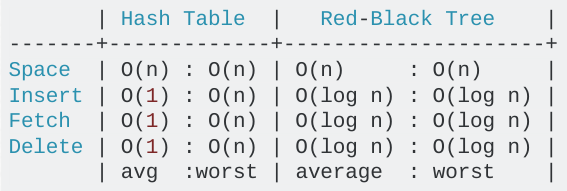
Python uses a hash table to get O(1) lookups on randomly accessed keys. The other most common choice for mapping objects is the binary tree lookup. Python's choice of the hash table over the B-tree was a conscious one.
Python’s dictionaries are implemented as resizable hash tables. Compared to B-trees, this gives better performance for lookup (the most common operation by far) under most circumstances, and the implementation is simpler. —python.org
In fact, you can see the performance difference very clearly:
When Keys Collide
The idea of a collision is one concept that can make or break a hash table implementation. Handling these properly for your use case can make your approach very fast. Handling them improperly can make things very slow.
Python hash had a history of problems with their approach to handling collisions that were worked out once and for all before Python 2.7. Going through these change sets is a phenomenal way to understand the shortcomings of various design decisions with respect to resolving collisions. To understand Python's approach to hash tables, it's important to know a little bit of terminology:
- hash: a numeric value a key is mapped to by a hashing algorithm. In other words; f(key) -> hash
- slot: an empty position in the hash table a dictionary key-value can possibly be saved to
- dummy key: when a key-value is deleted from a dictionary, we don't leave behind an empty slot. This would make it impossible to find other keys (we'll go into that later). We leave behind a dummy instead.
- NULL keys: the value a key has before a slot in the table is used/occupied by a key-value pair
- entry: a hash and a key-value pair occupying a slot
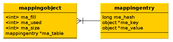
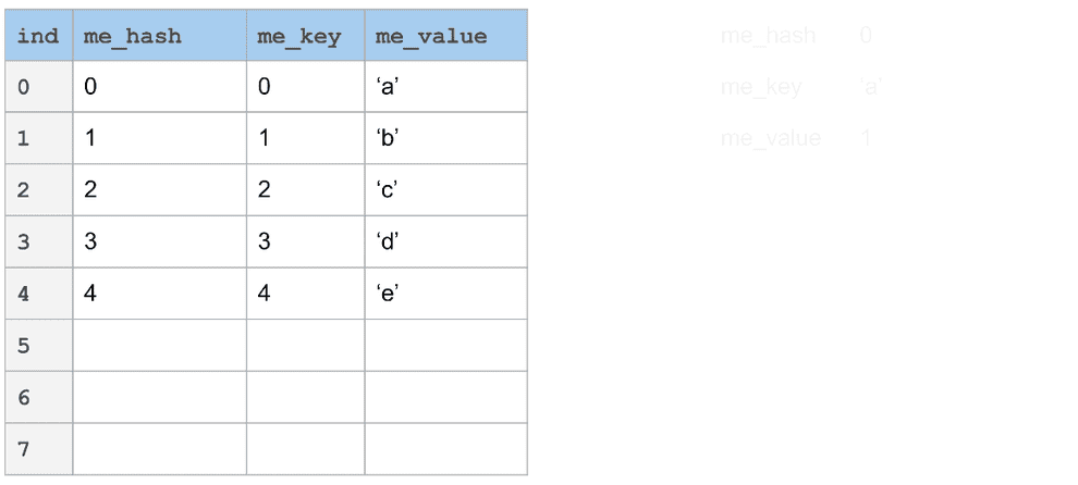
The mapping object is a container for mapping entry(s). It maintains a reference to ma_fill (the number of non-NULL keys — i.e., dummy keys + entries); ma_used (the number of non-NULL, non-dummy keys); and ma_size, a prime number representing the size (memory allocated) of the underlying table.
At the core of Python's lookup algorithm is a method called "lookmapping." Guido describes it in his commit as:
The basic lookup function used by all operations. This is essentially Algorithm D from Knuth Vol. 3, Sec. 6.4. Open addressing is preferred over chaining since the link overhead for chaining would be substantial.
Now that we have the building blocks, let's understand the difference between Open Addressing and Chaining. I'll explain below, but you're encouraged to have a look at the Wikipedia pages linked to above. Knuth's books are also available on Amazon if you're interested in picking up a copy.
Open Addressing
In Open Addressing, we allocate our whole address space. This includes space for all the entries we are able to insert directly into the space, as well as those that find their slot through a sequence of collisions.
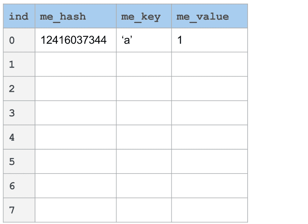
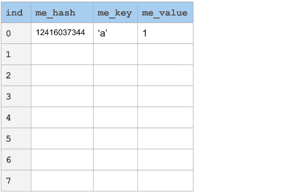
In the figure below, you'll see an example of a linear probe. The key 'a' hashes to 12416037344. Taking the modulo with the table size (8), we find it falls into slot 0. What if we want to add 'i' now, which would also map to slot 0? It's as simple as jumping forward some number of slots according to "incr." In our case, incr is set to 3. Each key that might collide with slot 0 will find its home n times incr away, where n is the number of collisions that have occurred up to that point.
The scenario we've described here has O(1) lookups in the best case, and O(n) in the worst. In the worst case, it amounts to a linear search of the space.
Chaining
Open Addressing differs from chaining in the way memory is allocated. Rather than probing for a new slot when a collision occurs, we just append to a linked list. This also has O(1) lookups in the best case, and O(n) in the worst. The major difference is the allocation overhead. In chaining, we have the additional operation of allocating an element on the heap for every collision that occurs during an insert operation.
Clustering
The quality of a hash table implementation in many ways comes down to the quality of its collision resolution mechanism. If keys become too close together in the table, we end up with a situation called "clustering." Clusters can make it likely there will be more than usual collisions over a range of keys and are, hence, typically undesirable.
Python's actual probe formula at the onset was as shown above: (3 * hash + 1) % table_size. Above is a real scenario depicted where we would have a linear cluster and very poor lookup performance.
OK. But really. What's the problem? Well, on January 16, 1997, Guido wrote this gem, with an acknowledgement that the core algorithm behind the dict lookup must be AFAP.
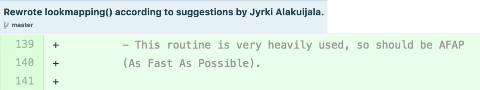
Clearly, at this time, it was not.
In modern implementations of GCC and clang, you'll find the modulo operation is optimized. But once upon a time, it actually broke down to this formula:
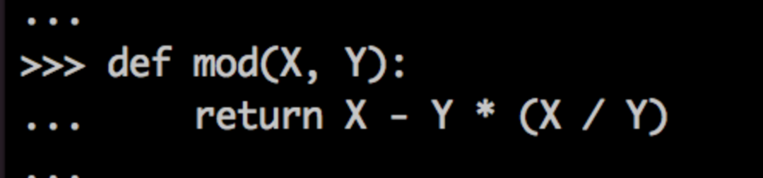
...which is three operations in one. Wow! To get away from this and move toward fewer, faster operations, Guido (with help from other contributors) committed a new lookup algorithm implementing the Galois Field for randomized lookups. This decreased the collision rate substantially.
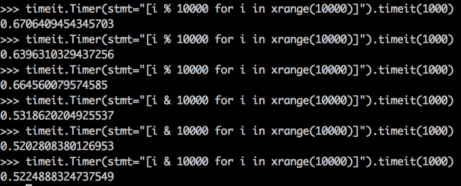
As a side note: In Python, the modulo operation is still a little slower than the bitwise & (which provides similar functionality).
Anyway, after the Galois Field, there were a series of minor changes to the lookmapping method that resulted in a 100% speed improvement. Have a look at the commit. It's very Death by a Thousand Cuts.
For those of you having trouble picking out what was changed, they
- changed sequences of "if" statements to "if/else";
- postponed casting "hash" until it was needed; and
- stored "hash" in a register instead of on the stack.
After these changes spent some time in the community for a few years, it was brought up on the python-dev list that not all the bits of the hash are actually coming into play when computing what slot an entry should be placed in.
One set in particular resulted in all entries landing in the same slot. That's the set defined by [i << 16 for i in range(20000)]. Consider the following commit message from the cpython project:
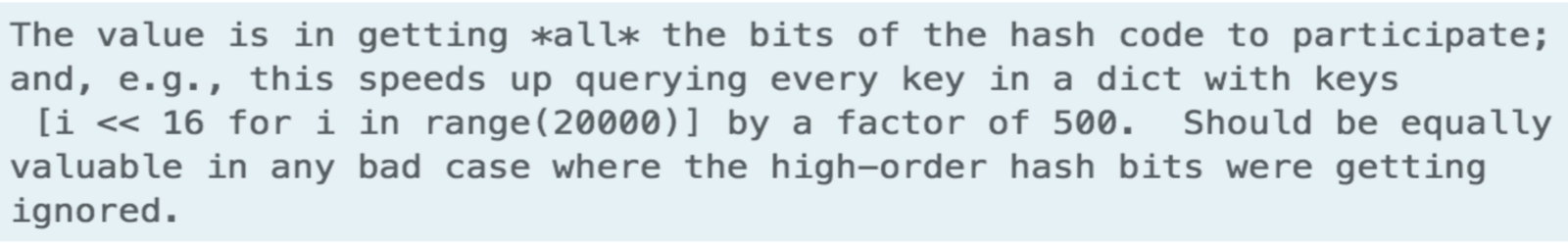
If the table size doubles every time (for the set mentioned above), every single entry is placed in slot 0. That's pretty bad. To fix this, Tim Peters committed a feature in May 2001 that uses polynomial division to incorporate more bits of the hash value with each subsequent collision.
I suppose the team thought this was a little difficult to understand. I'm not sure why, but a month later, on June 1, 2001, the polynomial division approach was stripped out for a pretty simple recurrent function.
To quote the comments in dictobject.c: At this point, the first half of collision resolution is to visit table indices via this recurrence...
j = ((5*j) + 1) mod 2**i
For any initial j in range(2**i), repeating that 2**i times generates each int in range(2**i).
Again from dictobject.c: The other half of the strategy is to get the other bits of the hash code into play. This is done by initializing an (unsigned) variable "perturb" to the full hash code and changing the recurrence to:
At this time, the following rules were solidified:
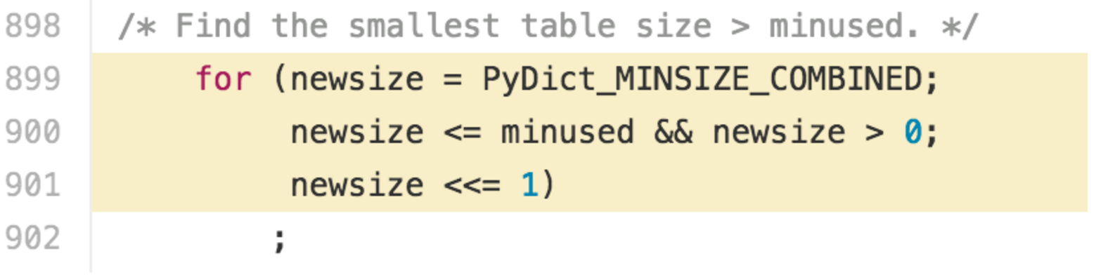
- Table size is 2**n, with a minimum size of 8 slots.
- Table indices are computed from hashes using the same number of hash bits as there are bits in the table size.
- Load factor (number of filled slots) must be below 2/3 table size or the table resizes to the next power of two.
Takeaways
OK. We just went through a lot of implementation. It's kind of nice to take something practical away from all this that you can use in your day-to-day. Here are a few things that fall directly out of what we reviewed.
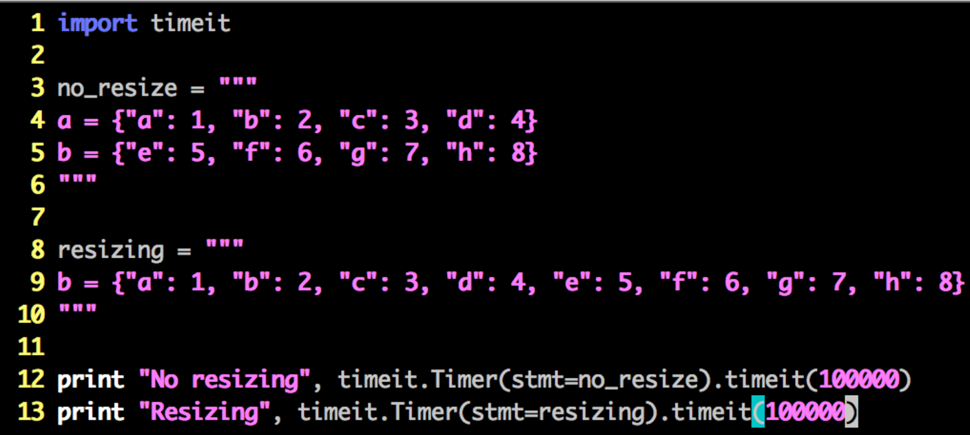
Resizing Is Not "Free"
Our default table size is 8 elements. Since the load factor must remain below 2/3, our table will resize upon adding a 5th element. Let's have a look at the difference between instantiating two 4-element dicts versus one 8-element dict.
You might expect the two 4-element dicts to take longer because of the overhead associated with creating two separate containers. That happens not to be the case. Consider the following code:
The output appears as
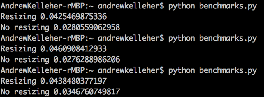
...indicating about a 30% performance benefit to avoiding resizing.
Now, in the words of Donald Knuth, "premature optimization is the root of all evil." I'm certainly not advocating splitting up logically related dicts to get speed improvements. If you're worried about such small speed improvements, you should probably consider pypy or another language altogether. On the other hand, if you have a database query, for example, you may consider replacing your SELECT * with just the elements you need (if you're not already).
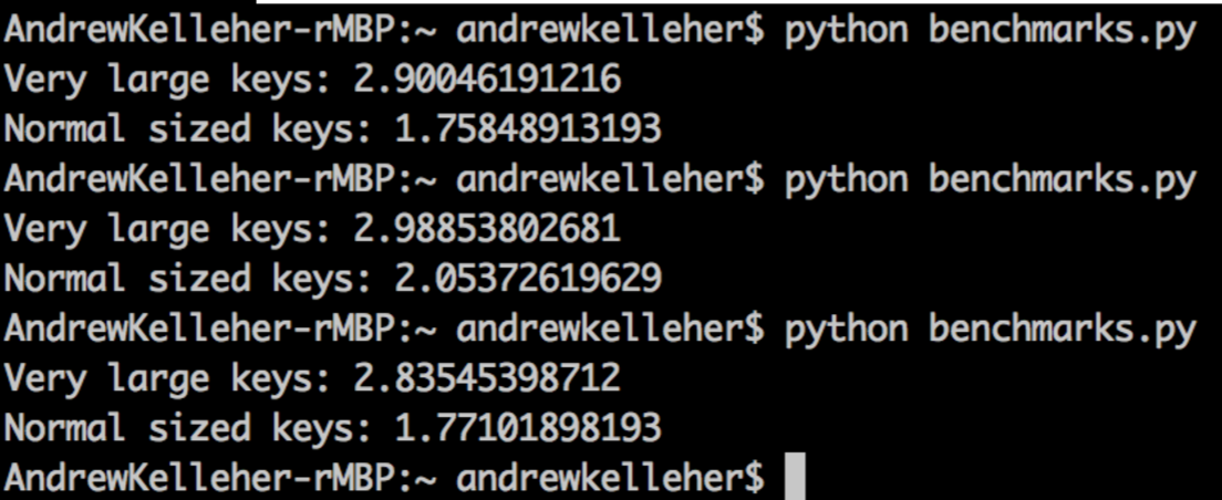
Small Keys Are Better Than Large Ones
We saw the 500-fold improvement for the set of integers bit-shifted 16 times. What about 32 times? Sounds crazy, right? 1 << 32 is in the 4B range. That's large but not astronomical. In fact, some schemes for assigning user IDs borrow from this range.
Consider the following code:
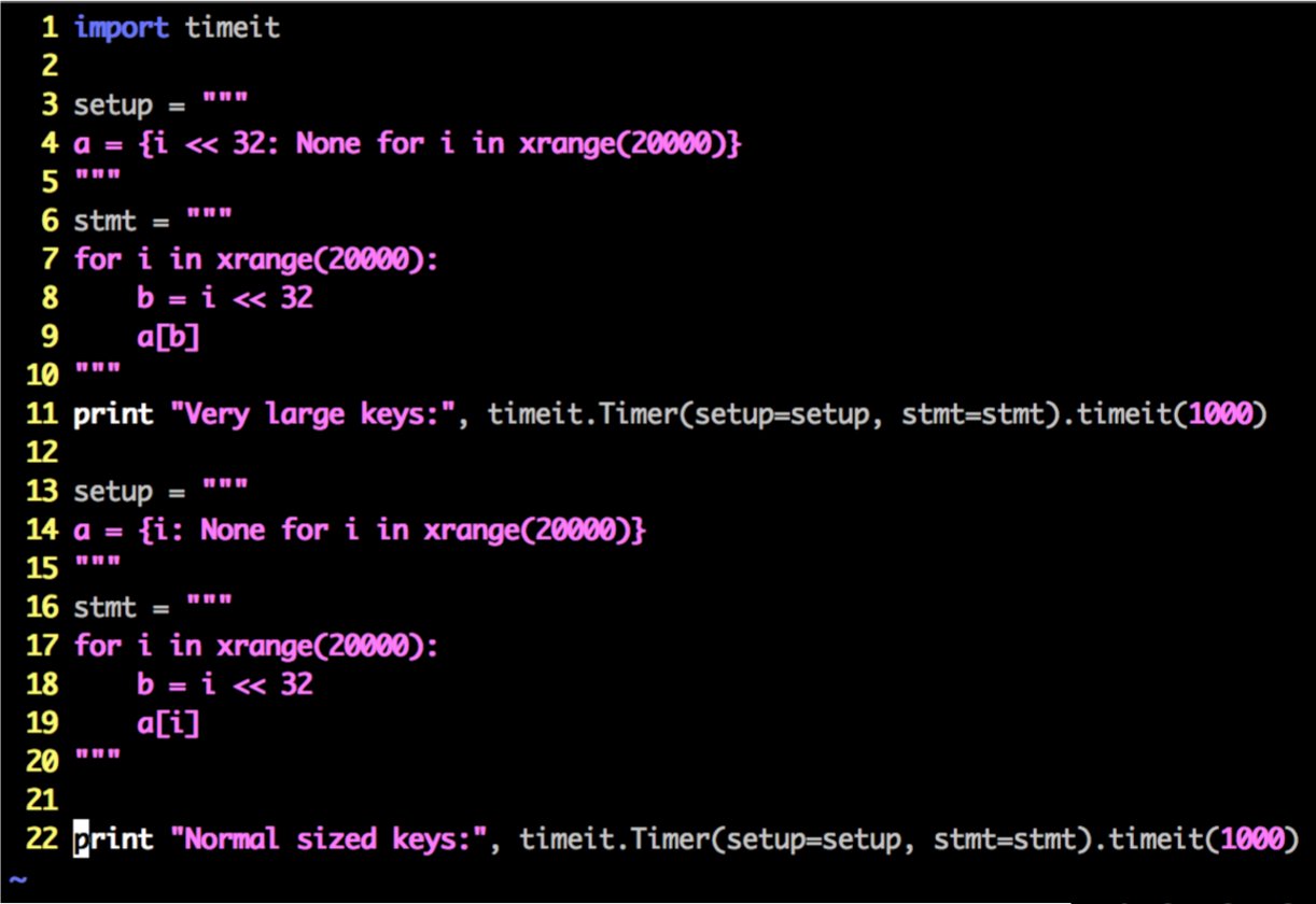
As you might have guessed from the context, the dict with very large keys takes about 30% longer to assign to, indicating a much higher rate of collisions.
Dicts Can Waste a Lot of Memory
Since the resizing plan for dicts follows the standard exponential (2**n) procedure, a dict slightly greater than 2/3 full can use quite a lot of extra space when it resizes.
Order Matters
People have probably told you the order of a dict is not guaranteed. That's true! But it actually is...kind of. The methods that calculate keys and place elements in the dict in cpython are deterministic. That means passing the same values will have the same results each time.
What causes elements to go out of order is actually the history of the dict. Consider the following.
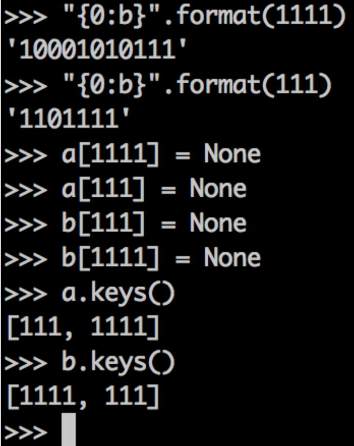
In this example, we have two keys: 1111 and 111. Since our table size is 8 (the default for a new dict), we know only three bits will be taken into account to place an element in the table (since there are 8 possible combinations of three bits).
Knowing that, we can hash them. The last three bits of each is 111, which means we'll have a collision for sure. Adding them to dict a in one order and to dict b in another order ensures the first element gets the first slot in the dict. When we try to add the next element, we'll have a collision, and it will be placed at another slot in the table (which happens to be before the first slot in this case).
When we print the keys of the dict, then, they're out of order. This behavior is consistent, though, and reproducible. As long as we add the elements in the same order, the order will be the same for the latest versions of python 2.7 and 3.x as of the time of this writing.
Dict Keys Should Be Treated As Immutable
For those of you who haven't tried, this is what happens when you attempt to use a mutable type as a key for a dict:
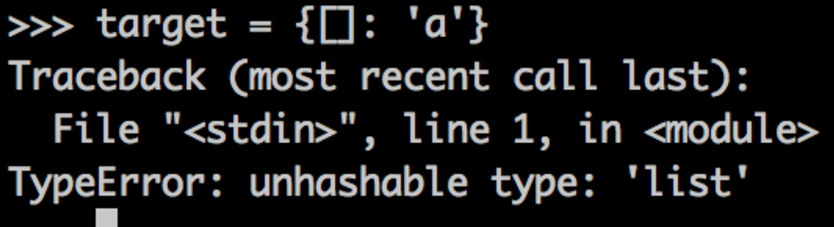
The problem here stems from the fact that mutable types don't have a __hash__() method by default. There is no inherent reason for this for a given container, but when you consider what __hash__() is used for, there's a great reason.
If you add a list as a key for a dict, then you mutate it; the hash will change. This means future lookups for that element will fail because passing the value to look up will have a different hash. Let's see an example.
First, we have to extend list with a class that defines a __hash__() method. This will do just fine.
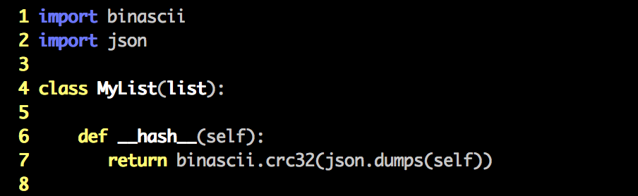
Now we can use our list as a mutable dict key! hlist is our hashable list. hlist2 is a separate hashable list containing the same elements.
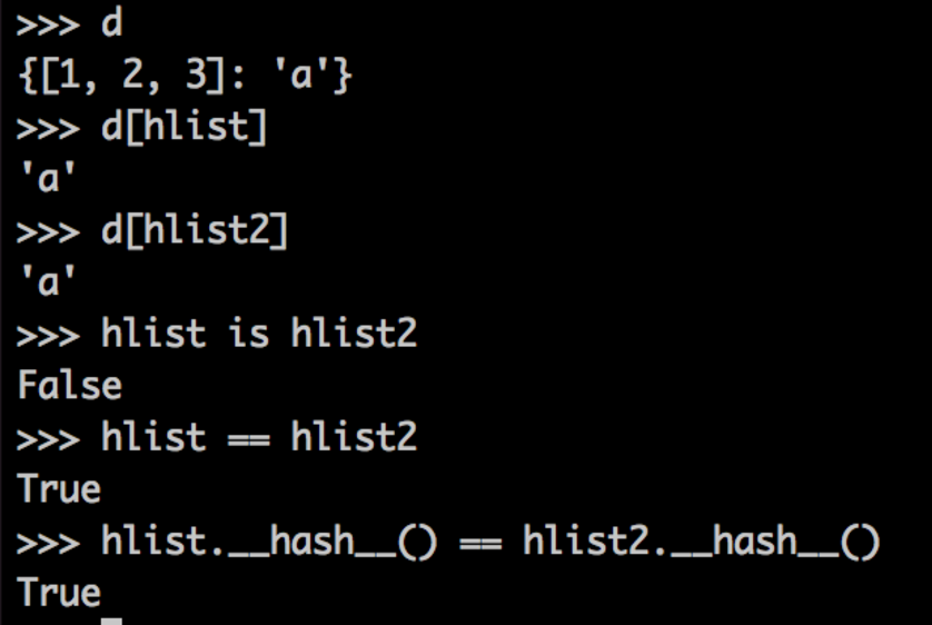
Setting d[hlist] = 'a', we can look up the value 'a' with either hlist or the new list, hlist2 (which contains the same values in the same order).
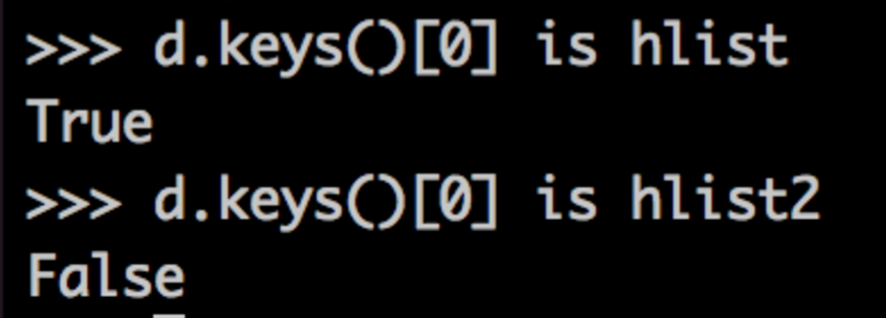
This is because the lists are the same by value, and they have the same output under __hash__(). Now let's mutate hlist. To be clear: The key of d that yields a is hlist. It's not the value of hlist, but hlist itself.
Modifying hlist by reference, then, will have some ill effects. This will cause the value of hlist to change as well as the hash. It's already in its assigned slot, though, which will most likely be inappropriate given its new hash and value.
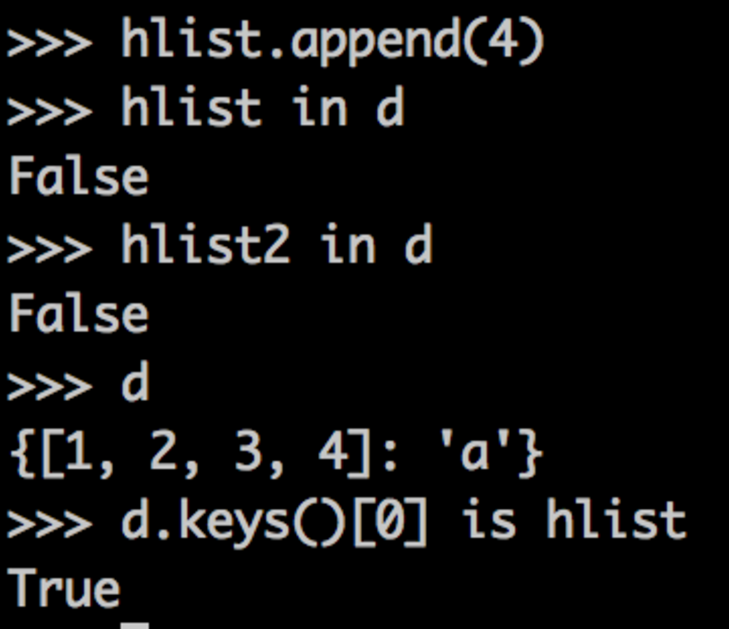
So, as you might expect, appending 4 to hlist causes lookup errors. It still exists in d as a key, but now it has a different hash and a different value.
When our lookup by the original variable, hlist, runs, we calculate the wrong hash, and it appears hlist is no longer in d. When we do the lookup by the original value, hlist2, we find the correct slot based on its hash, but the value doesn't match, so it appears hlist2 is not in d.